


I wrote an article on getting into 3D printing for mathematicians which was published in the Mathematical Intelligencer. The final publication is available at www.springerlink.com, at this page. A preprint is available here. This page contains additional notes and resources for that article.
Mathematica Code
Here is the mathematica code from the article, to save you typing it out.
f[u_, v_] := {u, v, u^2 - v^2};
scale = 40;
radius = 0.75;
numPoints = 24;
gridSteps = 10;
curvesU = Table[scale*f[u, i], {i, -1, 1, 2/gridSteps}];
curvesV = Table[scale*f[j, v], {j, -1, 1, 2/gridSteps}];
tubesU = ParametricPlot3D[curvesU, {u, -1, 1}, PlotStyle -> Tube[radius, PlotPoints -> numPoints], PlotRange -> All];
tubesV = ParametricPlot3D[curvesV, {v, -1, 1}, PlotStyle -> Tube[radius, PlotPoints -> numPoints], PlotRange -> All];
corners = Graphics3D[Table[Sphere[scale f[i, j], radius], {i, -1, 1, 2}, {j, -1, 1, 2}], PlotPoints -> numPoints];
output = Show[tubesU, tubesV, corners]
Export["MathematicaParametricSurface.stl", output]
Detailed instructions for making your 3D printed model with Shapeways
- Use your web browser to sign up for an account at shapeways.com.
- Upload your STL file to their servers. Currently, there is a tab on their website titled "create", under which the "upload" link is available.
- You will be asked to choose a unit of measure, and should choose "Millimeters" to be consistent with our scale calculations.
- After the upload is complete, you should receive an email confirming the upload of the file. If everything has gone through correctly, shortly afterwards you should receive a further email confirming that the model has passed Shapeways' automated checks (at this stage, their software deals with the multiple overlapping closed meshes).
- Next, you should be able to go to a webpage for your model and add it to your shopping cart. There will be a large selection of materials to choose from. I recommend using the option labelled "White Strong & Flexible". This is nylon plastic, 3D printed using a process called "selective-laser-sintering" (often referred to as SLS). The material is inexpensive and (as the name implies) very strong, and is flexible rather than brittle. At the time of writing, the model generated in this article costs less than US$10 in this material. Other materials (e.g. metals, glass, ceramics) have different requirements in terms of the minimum safe thickness of walls and tubes and so on. These requirements are documented on the website.
- After choosing your material and adding the model to your shopping cart, continue just as you would with any other online shopping service.
- Depending on where you are in the world, you can expect your 3D print(s) to arrive in the mail in a couple of weeks!
The webpage for my version of the model is here.
Going further
Using Mathematica
Unfortunately, Mathematica's point, line and curve graphics primitives cannot currently be exported to an STL file, even if you put a tube around them. The ParametricPlot3D technique used above is a work-around for this limitation. However, the 3D graphics primitive "Cylinder" does work, and could be used to make straight lines in your design.
The information in the rest of this section is mostly specific to Rhinoceros as it is the program I am most familiar with.
Polygonal meshes and NURBS surfaces
Mathematica outputs 3-dimensional geometry as a polygon mesh. In contrast, many 3D design programs work both with meshes and also with objects called "NURBS surfaces"("NURBS" stands for "Non-uniform rational B-spline".). NURBS surfaces are generalisations of Bézier curves. Just as 2-dimensional vector graphics programs use Bézier curves to represent smooth curves, 3D graphics programs represent smooth surfaces using NURBS surfaces. My usual workflow is to design a model using NURBS surfaces and then at the last step convert the NURBS surfaces into meshes, which can then be sent to a 3D printer. At the conversion step one can specify the fidelity with which the mesh approximates the NURBS surfaces.
Useful functions for Rhinoceros
If I were to make the same model as made by the above Mathematica code, but in Rhinoceros, I would use the function called "Pipe". This function takes input a 1-dimensional curve and outputs a pipe around it, in the form of a NURBS surface. This does the same job as the "Tube" directive in Mathematica. Rhinoceros doesn't have direct support for arbitrary parametric curves, but it can produce a curve which interpolates smoothly along a path of given points, and so one can build a curve which follows a desired parametric curve to very good precision. (To be fair, Mathematica and any other computer program is essentially doing this whenever it represents a curve graphically.)
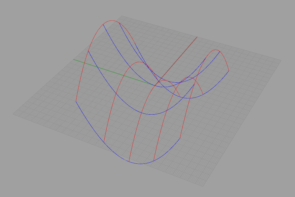
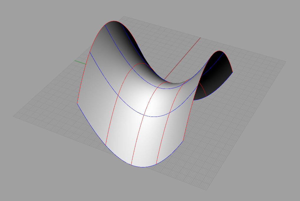
Another very useful tool in Rhinoceros is a function called "NetworkSrf". This takes as input two sets of curves, arranged as a combinatorial grid, so each curve from the first set meets each curve from the second set transversely in one point. The function returns a NURBS surface which smoothly interpolates between all of the curves. See the Figures to the right. Before we have two sets of curves arranged in a combinatorial grid, and then after, the NURBS surface generated by NetworkSrf.
We can build a closed surface out of these parameterised surface patches. This gives a large amount of control over the shape of the object, and is how many of my designs are constructed.
One potential pitfall to be aware of in this strategy is that the edges of the NURBS surface patches must match up precisely, and these surfaces must be "joined" in the program (using the "Join" command), meaning that we tell it that the edges between neighbouring patches are identified. At the stage when the NURBS surface is converted to a mesh, the program makes the polygonal approximations of the two joined edges identical. If the edges are not explicitly joined, this will not happen, and the resulting polygonal mesh will not be closed. An easy way to make the edges of the surface patches match precisely is to generate the surface patches using the exact same curve at the edges. Note that this will not necessarily happen if taking advantage of a symmetry of the object: a rotated or reflected curve might not match precisely due to floating point errors, and so may not be possible to join.
Recently, I have also had trouble with matching surface patches generated using arcs of circles. Using "AddInterpCurve" with a few hundred points seems to work better.
Dealing with non-embedded meshes
The Mathematica code, and many other constructions give a number of closed polygonal meshes that overlap with each other. 3D printers generally require disjoint closed meshes. In order to fix this, we need to view each of the closed polygonal meshes as describing a solid with polygonal boundary, take the union of these solids and then produce the boundary of the union as a polygonal mesh. Rhinoceros and Blender both have functions to perform this operation (called "Boolean union" in these programs), although they sometimes have trouble with complicated geometry. Another useful option is the software provided by a company called "netfabb". Their programs are specifically designed for preparing meshes for 3D printing. They currently provide a free online service at http://cloud.netfabb.com/, which attempts to take the appropriate unions and otherwise fix problems with a mesh. Even this software can sometimes fail when faces of the polygonal solids are coincident, and it may be necessary to fix problems with a mesh by hand.
Reducing the polygon count
Depending on how you make your mesh, you may end up with a large file with many thousands, or even millions of polygons. Shapeways currently has a limit of 1 million polygons for files that it will accept. There are a few options available for reducing the number of polygons without sacrificing (much) quality. Two opensource programs that I have used for this are MeshLab and OpenFlipper. In MeshLab, use "Filters > Remeshing, simplification and construction > Quadratic Edge Collapse Detection", and in OpenFlipper, use "Decimater".
Further price considerations
There can be multiple ways to represent a mathematical object, some more expensive than others. In the article for example, we discussed a surface represented as a grid, or as the whole surface (which would be more expensive). Sometimes it is necessary to have the whole surface, as in the solid of constant width in the article. The object wouldn't roll correctly if it was represented as a grid. However, for solid objects like this, it is a very good idea to hollow it out, making only a shell of the object. Usually, you will want to make at least one hole in the surface so that scaffolding material can be removed from the interior of the shell.
If a design turns out to be too expensive, a small reduction in scale can go a very long way. With Shapeways at least, they generally charge by volume of material used. Therefore, in order to halve the cost one needs to scale by a factor of the cuberoot of 0.5, or just under 0.8, which won't make a huge difference to the look of the object. Of course, this doesn't work so well if features of your design are already at the minimum printable thickness.